The objective of the Exploratory Data Analysis (EDA) is to check all the data sets available, evaluate if there is a need to clean and process the data further to be able to model and evaluate if there are patterns that I need to take into account.

This EDA will be divided into two main sections: Santa Rosa National Park data and MODIS derived data.

SRNP data exploration

Santa Rosa National Park Environmental Super Site in Guanacaste, Costa Rica have several sensors to monitor environmental climate variables and fluxes.

Given that variables such as NDVI and GPP can be calculate with instrumentation in the site, this ones will be included and name as in-situ_variable_name to differentiate them from the same variables obtained from the MODIS satellite images.

The following table shows the data sets used to conduct this research. There are 3 different data sets which contains variables of interest. Not all data sets have the same time range or the same time frequency for each observation:

Dataset	Frequency	Date range
Precipitation	Daily values	`2013-05-15 00:00:00 UTC` to `2017-05-17 23:30:00 UTC`
Meteorological data	Half hour values	`2013-05-15 00:00:00 UTC` to `2017-05-17 23:30:00 UTC`
Monthly Gross Primary Production (GPP)	Monthly values	`2013-05-01` to `2017-05-01`

Santa Rosa Data tables glimpse

This section contains tables that shows the first 100 rows and all the variables contained in each of the data sets shown in the table above:

Precipitation data

Show code

precipitation %>% 
  slice(1:100) %>% 
  paged_table()

Meteorological data

Show code

biomet %>% 
  slice(1:100) %>% 
  paged_table()

Monthly GPP in-situ data

Show code

monthly_gpp %>% 
  slice(1:100) %>% 
  paged_table()

Show code

ndvi_moha %>% 
  slice(1:100) %>% 
  paged_table()

Precipitation seasonal patterns

The total annual precipitation in Santa Rosa National Park is between 700 and 2000 mm, with a dry season of 4 to 5 months where precipitation is less than 100 mm per month or even 0 mm (Sánchez-Azofeifa et al., 2005). For the time period of this research, the site experimented a drought season in 2014 and 2015 (Castro et al. 2018)

Show code

precipitation %>% 
  mutate(year_mon = zoo::as.yearmon(date)) %>% 
  group_by(year_mon) %>% 
  summarize(
    total_precip = sum(precip, na.rm = TRUE)
  ) %>% 
  ggplot(aes(x = as.factor(year_mon), y = total_precip)) +
  geom_bar(stat = "identity") +
  theme_light() +
  theme(axis.text.x = element_text(angle = 90, h = 1)) +
  labs(x = "Date", y = "Total precipitation per month (mm)")

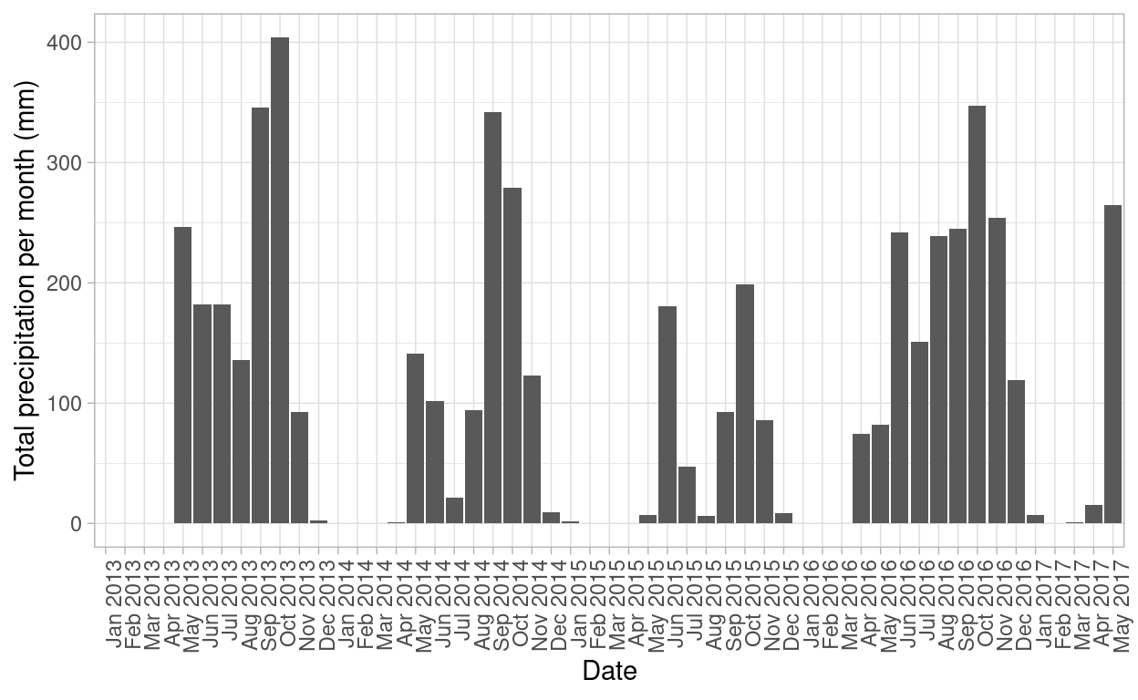
Figure 1: Total precipitation (mm) for Santa Rosa National Park. Year 2015 had the lowest values of precicipitation

Show code

### Agrupando los meses
precipitation %>%
  mutate(year_mon = zoo::as.yearmon(date)) %>%
  filter(year(date) < 2017) %>% 
  group_by(year_mon) %>%
  summarize(
    total_precip = sum(precip, na.rm = TRUE)
  ) %>%
  mutate(year = year(year_mon),
         month = month(year_mon, label = TRUE)) %>%
  # mutate(year_mon = as.character(year_mon)) %>%
  ggplot(aes(x = as.factor(month), y = total_precip, fill = as.factor(year))) +
  geom_bar(stat = "identity", position = "dodge") +
  theme_light(base_size = 12) +
  scale_y_continuous(breaks = seq(0, 450, by = 50)) +
  scale_fill_viridis_d() +
  labs(x = "Date", y = "Total precipitation per month (mm)",
       fill = "Year")

Metereological variables

From the site, there is instrumentation to measure environmental variables such as Vapor Pressure Deficit (VPA), Air Temperature (TA), Latent Heat (LH), relative humidity (RH) and Soil Water Content (SWC). In order to explore these variables, I plotted them with box plots to check the variability outliers and patterns per month, across all the time range available (May 2013 to May 2017).

Show code

vpd_plot <- biomet %>% 
  mutate(year_mon = zoo::as.yearmon(date)) %>% 
  filter(vpd > 0) %>% 
  ggplot(aes(x = as.factor(year_mon), y = vpd)) +
  geom_rect(aes(xmin = "Jan 2015",
                xmax = "Jan 2016",
                ymin = 0,
                ymax = Inf),
            alpha = 0.05,
            fill = "#D8E082") +
  stat_boxplot(geom = "errorbar", width = 0.25) +
  geom_boxplot() +
  scale_y_continuous(breaks = seq(-10, 40, by = 5)) +
  scale_fill_viridis_d() +
  theme_light(base_size = 10) +
  theme(axis.text.x = element_text(angle = 90, h = 1)) +
  guides(fill = "none") +
  labs(x = "Date", y = "VPD (hPa)")

at_plot <- biomet %>% 
  mutate(year_mon = zoo::as.yearmon(date)) %>%
  ggplot(aes(x = as.factor(year_mon), y = tair)) +
  geom_rect(aes(xmin = "Jan 2015",
                xmax = "Jan 2016",
                ymin = 15,
                ymax = Inf),
            alpha = 0.05,
            fill = "#D8E082") +
  stat_boxplot(geom = "errorbar", width = 0.25) +
  geom_boxplot() +
  scale_y_continuous(breaks = seq(15, 38, by = 2)) +
  scale_fill_viridis_d() +
  theme_light(base_size = 10) +
  theme(axis.text.x = element_text(angle = 90, h = 1)) +
  guides(fill = "none") +
  labs(x = "Date", y = "TA (C)")

lh_plot <- biomet %>% 
  mutate(year_mon = zoo::as.yearmon(date)) %>%
  filter(le > 0) %>%
  ggplot(aes(x = as.factor(year_mon), y = le)) +
  geom_rect(aes(xmin = "Jan 2015",
                xmax = "Jan 2016",
                ymin = 0,
                ymax = Inf),
            alpha = 0.05,
            fill = "#D8E082") +
  stat_boxplot(geom = "errorbar", width = 0.25) +
  geom_boxplot() +
  scale_fill_viridis_d() +
  theme_light(base_size = 10) +
  theme(axis.text.x = element_text(angle = 90, h = 1)) +
  guides(fill = "none") +
  labs(x = "Date", y = "LH (Wm-2)")

rh_plot <- biomet %>% 
  mutate(year_mon = zoo::as.yearmon(date)) %>%
  ggplot(aes(x = as.factor(year_mon), y = r_h)) +
  geom_rect(aes(xmin = "Jan 2015",
                xmax = "Jan 2016",
                ymin = 0,
                ymax = Inf),
            alpha = 0.05,
            fill = "#D8E082") +
  stat_boxplot(geom = "errorbar", width = 0.25) +
  geom_boxplot() +
  scale_fill_viridis_d() +
  theme_light(base_size = 10) +
  theme(axis.text.x = element_text(angle = 90, h = 1)) +
  guides(fill = "none") +
  labs(x = "Date", y = "RH (%)")

swc_plot <- biomet %>% 
  mutate(year_mon = zoo::as.yearmon(date)) %>%
  filter(swc > 0) %>%
  ggplot(aes(x = as.factor(year_mon), y = swc)) +
  geom_rect(aes(xmin = "Jan 2015",
                xmax = "Jan 2016",
                ymin = 0,
                ymax = Inf),
            alpha = 0.05,
            fill = "#D8E082") +
  stat_boxplot(geom = "errorbar", width = 0.25) +
  geom_boxplot() +
  scale_fill_viridis_d() +
  theme_light(base_size = 10) +
  theme(axis.text.x = element_text(angle = 90, h = 1)) +
  guides(fill = "none") +
  labs(x = "Date", y = "SWC (%)")


plot_grid(vpd_plot, at_plot, lh_plot, rh_plot, swc_plot,
          nrow = 5,
          labels = "AUTO",
          label_size = 10,
          align = "v"
)

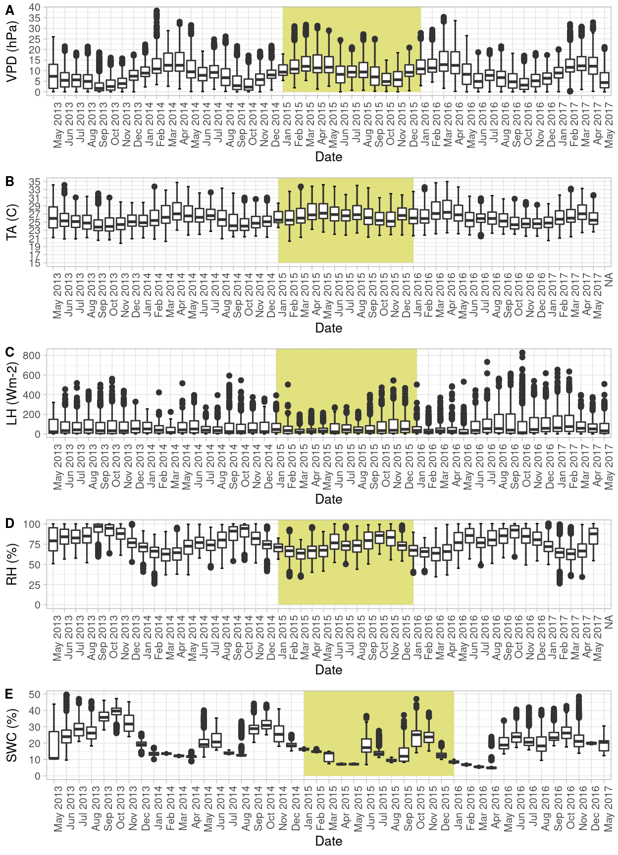
Figure 2: Seasonal pattern of environmental variables at Santa Rosa National Park. Yellow background denotes the year with less precipitation

Show code

ndvi_moha %>% 
  mutate(date = ymd(date)) %>% 
  filter(year(date) < 2017) %>% 
  ggplot(aes(x = date, y = ndvi)) +
  # geom_point(alpha = 0.5, color = "#FF3A1D", size = 3) +
  geom_jitter(alpha = 0.5, color = "#FF3A1D", size = 2.5) +
  theme_linedraw() +
  scale_x_date(date_labels = "%b%Y", breaks = "months") +
  theme(axis.text.x = element_text(angle = 90, h = 1))

Monthly GPP estimated in-situ

Monthly GPP values for the Santa Rosa National Park were obtained from the Harvard dataverse, as a result of the publication from Castro et al. 2018 were GPP was estimated using a light-response curve. Values presented here are the mean per month.

Show code

monthly_gpp %>% 
  ggplot(aes(x = date, y = average_gpp, group = 1)) +
  geom_errorbar(aes(ymin = average_gpp - gpp_stdev,
                    ymax = average_gpp + gpp_stdev),
                colour = "#4D4D4D", width = 20, size = 0.5) +
  geom_line(linetype = 2) +
  geom_point(color = "#FF3A1D", size = 3.5) +
  theme_linedraw() +
  scale_x_date(date_labels = "%b%Y", breaks = "months") +
  theme(axis.text.x = element_text(angle = 90, h = 1)) +
  labs(x = "Date", y = "GPP (mg m-2 s-1)")

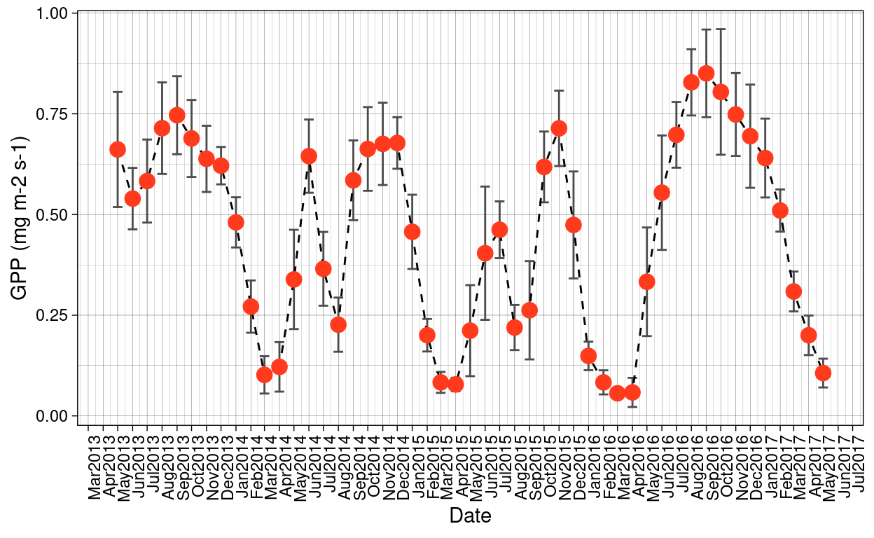
Figure 3: Monthly GPP values estimated in-situ for Santa Rosa National Park

Show code

ndvi_summarized <- ndvi_moha %>% 
  mutate(year_mon = zoo::as.yearmon(date)) %>% 
  group_by(year_mon) %>% 
  summarize(
    ndvi_mean = mean(ndvi, na.rm = TRUE),
    ndvi_sd = sd(ndvi, na.rm = TRUE)
  )

gpp_ndvi <- monthly_gpp %>% 
  mutate(year_mon = zoo::as.yearmon(date)) %>% 
  inner_join(ndvi_summarized) 

gpp_ndvi %>% 
  ggplot(aes(x = average_gpp, y = ndvi_mean)) +
  geom_point(color = "#FF3A1D", size = 3.5) +
  theme_linedraw() +
  geom_smooth(method = "lm")


model <- lm(average_gpp ~ ndvi_mean, data = gpp_ndvi)
# summary(model)
# report(model)

MODIS data exploration

MODIS data consist of 2 datasets: one with the GPP observations and a second one with the indices (NDVI and EVI) observations. In this section I will explore the data quality and possible relations between those variables.

MODIS data tables glimpse

Data derived from satellite images for Santa Rosa is compose of following data sets:

MODIS indices data

Show code

modis_indices %>% 
  slice(1:100) %>% 
  paged_table()

MODIS GPP data

Show code

modis_gpp %>% 
  slice(1:100) %>% 
  paged_table()

Observations per month

Show code

## This takes from 94 observations to 53 observations. Remove 41 observations
modis_indices_clean <- modis_indices %>% 
  filter(reliability_modland_description == "Good data, use with confidence") %>% 
  select(date, ndvi, evi) 

## Filter observations with good quality
## This takes from 183 observations to 114. Remove 69 observations.
modis_gpp_clean <- modis_gpp %>% 
  filter(modland_description == "Good quality",
         cloud_state_description == "Significant clouds NOT present (clear)",
         scf_qc_description == "Very best possible") %>% 
  select(date, gpp)

Given that satellite images from MODIS consist of at least 2 observations per month for the site, we need to evaluate how many data points I have for the analysis after filtering out observations with low quality (clouds present and image quality assurance flags marked as bad)

From MODIS I have two datasets (one composed with GPP observations and a second one composed with NDVI and EVI indices observations) the process was applied for both datasets. In the case of GPP I had in total 183 and after filtering observations without good data quality the total observations remaining are 114.

For the EVI and NDVI data set, originally I had 94 and after the filtering, I obtained 53 in total for further analysis.

Show code

modis_indices_clean %>% 
  group_by(zoo::as.yearmon(date)) %>% 
  tally() %>% 
  rename("date" = `zoo::as.yearmon(date)`, "total" = "n") %>% 
  ggplot(aes(x = as.factor(date),
             y = total))  +
  geom_bar(stat = "identity", fill = "#75AADB") +
  scale_y_continuous(breaks = seq(0, 3, by = 1)) +
  labs(x = "Date",
       y = "Total  MODIS indices observations") +
  theme_light(base_size = 10) +
  theme(axis.text.x = element_text(angle = 90, h = 1))

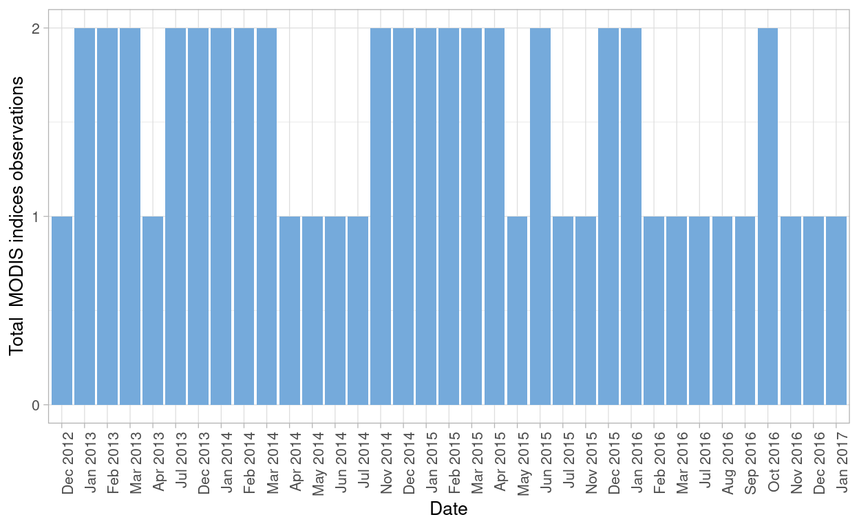
Figure 4: MODIS NDVI and EVI observations after filtering bad quality data points from both datasets

Show code

modis_gpp %>% 
  group_by(zoo::as.yearmon(date)) %>% 
  tally() %>% 
  rename("date" = `zoo::as.yearmon(date)`, "total" = "n") %>% 
  ggplot(aes(x = as.factor(date),
             y = total))  +
  geom_bar(stat = "identity", fill = "#75AADB") +
  scale_y_continuous(breaks = seq(0, 5, by = 1)) +
  labs(x = "Date",
       y = "Total  MODIS GPP observations") +
  theme_light(base_size = 10) +
  theme(axis.text.x = element_text(angle = 90, h = 1))

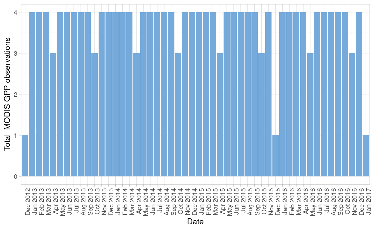
Figure 5: MODIS GPP observations after filtering bad quality data points from both datasets

GPP, NDVI, and EVI seasonal patterns

Given that the time range of the data set selected for this research goes from November 2012 to March 2017 and that Santa Rosa National Park presents a rainy season and a dry season, I want to check first if there those seasonal patterns are reflected in the MODIS products:

Show code

modis_gpp_clean %>% 
  ggplot(aes(x = date, y = gpp, group = 1)) +
  geom_line(linetype = 2) +
  geom_point(color = "#FF3A1D", size = 3.5) +
  theme_linedraw() +
  scale_x_date(date_labels = "%b%Y", breaks = "months") +
  theme(axis.text.x = element_text(angle = 90, h = 1)) +
  labs(x = "Date", y = "GPP (mg m-2 s-1)")

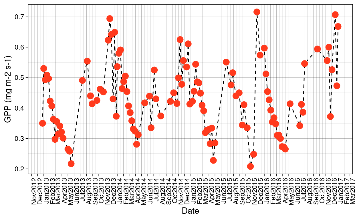
Figure 6: MODIS GPP trends over the time period

Show code

modis_indices_clean %>% 
  mutate(date = ymd(date)) %>% 
  filter(ndvi > 0.2) %>% 
  ggplot(aes(x = date, y = ndvi)) +
  geom_jitter(alpha = 0.7, color = "#FF3A1D", size = 3) +
  geom_line(linetype = 2) +
  theme_linedraw() +
  scale_x_date(date_labels = "%b%Y", breaks = "months") +
  theme(axis.text.x = element_text(angle = 90, h = 1)) +
  labs(x = "Date", y = "NDVI")

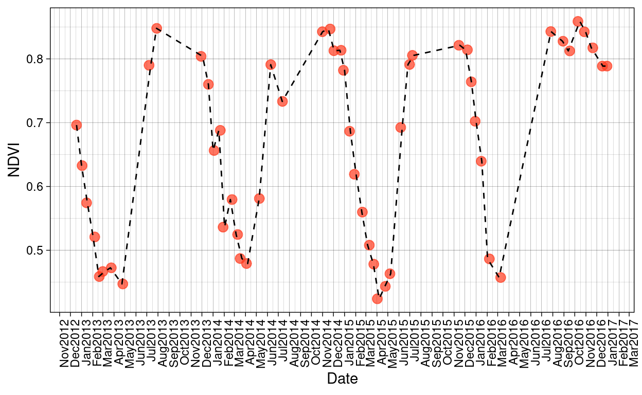
Figure 7: MODIS NDVI trends over the time period

Show code

modis_indices_clean %>% 
  mutate(date = ymd(date)) %>% 
  filter(ndvi > 0.2) %>% 
  ggplot(aes(x = date, y = evi)) +
  geom_jitter(alpha = 0.7, color = "#FF3A1D", size = 3) +
  geom_line(linetype = 2) +
  theme_linedraw() +
  scale_x_date(date_labels = "%b%Y", breaks = "months") +
  theme(axis.text.x = element_text(angle = 90, h = 1)) +
  labs(x = "Date", y = "EVI")

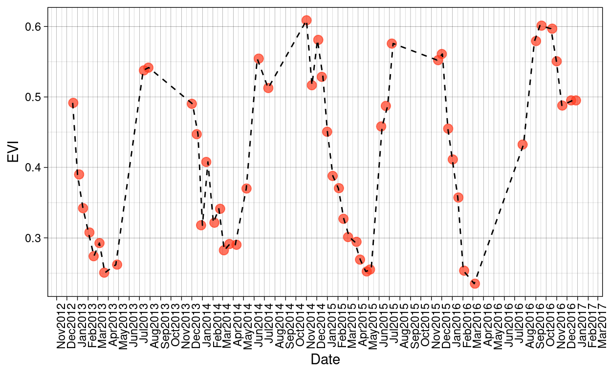
Figure 8: MODIS EVI trends over the time period

What is the relation between EVI NDVI & GPP MODIS products?

Show code

## Filter observations with good quality
## This takes from 94 observations to 53 observations. Remove 41 observations
modis_indices_clean <- modis_indices %>% 
  filter(reliability_modland_description == "Good data, use with confidence") %>% 
  select(date, ndvi, evi) 

## Filter observations with good quality
## This takes from 183 observations to 114. Remove 69 observations.
modis_gpp_clean <- modis_gpp %>% 
  filter(modland_description == "Good quality",
         cloud_state_description == "Significant clouds NOT present (clear)",
         scf_qc_description == "Very best possible") %>% 
  select(date, gpp) 

modis_join <- modis_gpp_clean %>% 
  full_join(modis_indices_clean, by = c("date"))

We are using products from MODIS which are: EVI, NDVI and GPP. These are already calculated values that are available to users. These products comes with variables that flags low quality values. In this case we have a data set with flags for GPP and a data set with flags for the indices EVI and NDVI.

All values with flags that advertised low quality data points were remove from both data sets. Then a pearson correlation was performed to explore the relation between GPP and NDVI, and GPP with EVI.

As validation for the relations between products from MODIS, I proceed to compare NDVI and EVI against GPP to check how is the relation between these variables.

Show code

#### Relation between NDVI and GPP from MODIS
gpp_ndvi <- modis_join %>% 
  ggplot(aes(x = ndvi, y = gpp)) +
  geom_point(color = "#FF3A1D", size = 3.5) +
  geom_smooth(method = "lm", color = "#4E5C68") +
  theme_light(base_size = 12) +
  # theme(axis.text.x = element_text(angle = 90, h = 1)) +
  labs(x = "NDVI", y = "GPP (mgm-2s-1)")

#### Relation between EVI and GPP from MODIS
gpp_evi <- modis_join %>% 
  ggplot(aes(x = evi, y = gpp)) +
  geom_point(color = "#FF3A1D", size = 3.5) +
  geom_smooth(method = "lm", color = "#4E5C68") +
  theme_light(base_size = 12) +
  # theme(axis.text.x = element_text(angle = 90, h = 1)) +
  labs(x = "EVI", y = "GPP (mg m-2 s-1)")

## Arrange both plots in one figure:
plot_grid(gpp_ndvi, gpp_evi, labels = c('A', 'B'), label_size = 12)

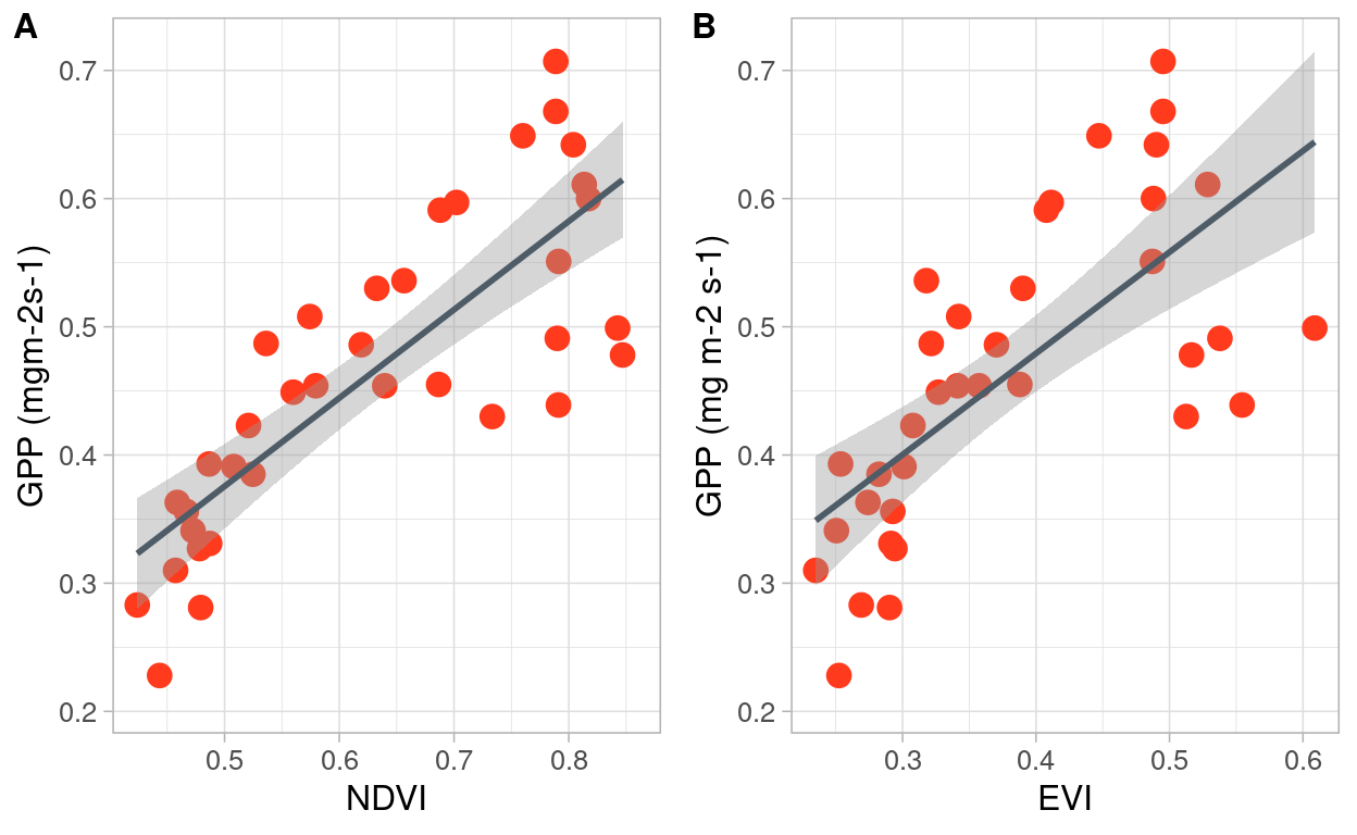
Figure 9: Relation between NDVI and GPP products from MODIS for the Santa Rosa National Park

Show code

ndvi_corr_test <- cor.test(modis_join$ndvi, modis_join$gpp)
evi_corr_test <- cor.test(modis_join$evi, modis_join$gpp)

# Check the report of the result
# report(ndvi_corr_test)
# report(evi_corr_test)

The Pearson’s product-moment correlation between NDVI and GPP products from MODIS is positive and statistically significant. (r = 0.81, 95% CI [0.65, 0.90], t(34) = 8.01, p < .001). For EVI and GPP the Pearson’s product-moment correlation is is positive, and statistically significant (r = 0.70, 95% CI [0.48, 0.84], t(34) = 5.70, p < .001)

MODIS NDVI, EVI & GPP trends over time

Show code

# Plot with both GPP's
rec_monthly_gpp <- monthly_gpp %>% 
  select(date, average_gpp) %>% 
  rename(gpp = average_gpp) %>% 
  mutate(origin = "in_situ")

rec_modis_gpp <- modis_gpp %>% 
  select(date, gpp) %>% 
  mutate(date = floor_date(date, "month")) %>% 
  group_by(date) %>% 
  summarise(
    gpp = mean(gpp, na.rm = TRUE)
  ) %>% 
  mutate(origin = "modis") %>% 
  filter(date > ymd("2013-04-30"))

rec_both <- bind_rows(rec_monthly_gpp, rec_modis_gpp)

## Correlation trends between both GPP's`
rec_both %>% 
  ggplot(aes(x = date, y = gpp, group = origin)) +
  geom_line(aes(color = origin), size = 1) +
  theme_light(base_size = 10) +
  scale_x_date(date_labels = "%b%Y", breaks = "months") +
  theme(axis.text.x = element_text(angle = 90, h = 1)) +
  labs(x = "Date", y = "GPP (mg m-2 s-1)", color = "GPP source")

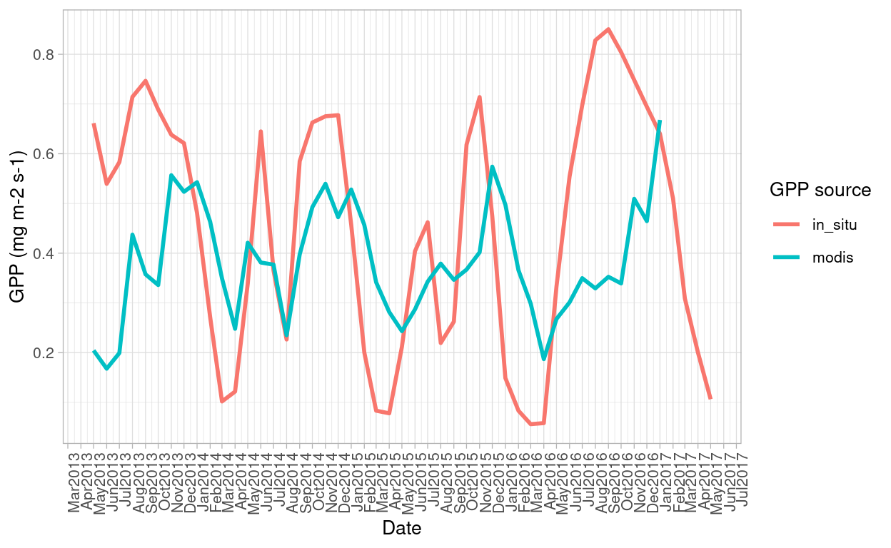
GPP trends over the years for MODIS and in-situ data. Despite having similar trends, range is higher for in-situ data than the MODIS derived GPP

Figure 10: GPP trends over the years for MODIS and in-situ data. Despite having similar trends, range is higher for in-situ data than the MODIS derived GPP

Summary

This is a bullet list with the main insights from the exploratory data analysis that can help to understand the models and the phenomena explained in the Results and Discussion section

NDVI have a higher positive correlation with GPP product from MODIS than EVI.
Year 2015 was the lowest year in precipitation
GPP estimated in-situ does not match the pattern of GPP obtained from the MODIS product.

References

Castro, S. M., Sanchez-Azofeifa, G. A., & Sato, H. (2018). Effect of drought on productivity in a Costa Rican tropical dry forest. Environmental Research Letters, 13(4), 045001.

Sánchez‐Azofeifa, G. A., Quesada, M., Rodríguez, J. P., Nassar, J. M., Stoner, K. E., Castillo, A., … & Cuevas‐Reyes, P. (2005). Research priorities for Neotropical dry forests 1. Biotropica: The Journal of Biology and Conservation, 37(4), 477-485.