Results
What is the relation between MODIS products and GPP estimated in-situ?
We have two indices derived from MODIS that can have a relation with the estimation of GPP in-situ. A linear model was performed to evaluate the relation between NDVI with GPP and, EVI with GPP estimated in-situ.
The clean data sets from MODIS products were used here altogether with the GPP data set with the estimations per month from Santa Rosa National Park.
MODIS NDVI and GPP in-situ
Given that observations for GPP in-situ are one per month and we have in most cases for the same period of time, more than one observation from MODIS, I have summarized MODIS values with the mean per month. A linear regression was performed and residuals were evaluated to look for patterns.
Show code
## Prepare data for model
ndvi_gpp_in_situ <- modis_indices_clean %>%
  group_by(zoo::as.yearmon(date)) %>%
  summarise(
    ndvi_mean = mean(ndvi, na.rm = TRUE),
    evi_mean = mean(evi, na.rm = TRUE)
  ) %>%
  rename(month_year = `zoo::as.yearmon(date)`) %>%
  full_join(modis_in_situ_gpp, by = "month_year")

## Create the linear models and check results
ndvi_gpp_model <- lm(average_gpp ~ ndvi_mean, data = ndvi_gpp_in_situ)
evi_gpp_model <- lm(average_gpp ~ evi_mean, data = ndvi_gpp_in_situ)

## Report models results
# summary(ndvi_gpp_model)
# report(ndvi_gpp_model)
# plot(evi_gpp_model)
# summary(evi_gpp_model)
# report(evi_gpp_model)
Show code
ndvi_gpp <- ndvi_gpp_in_situ %>%
  ggplot(aes(x = ndvi_mean, y = average_gpp)) +
  geom_point(color = "#FF3A1D", size = 3.5) +
  geom_smooth(method = "lm", color = "#4E5C68") +
  theme_light(base_size = 12) +
  labs(x = "MODIS NDVI", y = "GPP (mg m-2 s-1)")

evi_gpp <- ndvi_gpp_in_situ %>%
  ggplot(aes(x = evi_mean, y = average_gpp)) +
  geom_point(color = "#FF3A1D", size = 3.5) +
  geom_smooth(method = "lm", color = "#4E5C68") +
  theme_light(base_size = 12) +
  labs(x = "MODIS EVI", y = "GPP (mg m-2 s-1)")

## Arrange both plots in one figure:
plot_grid(ndvi_gpp, evi_gpp, labels = c('A', 'B'), label_size = 12)
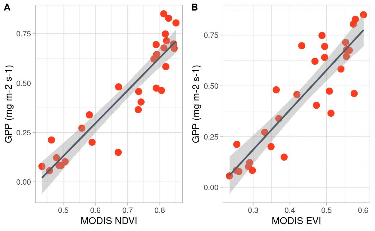
Figure 1: Relation between NDVI and EVI indices derived from MODIS with GPP estimated in-situ
I fitted a linear model (estimated using OLS) to predict GPP in-situ with MODIS NDVI product (formula: GPP in-situ ~ NDVI) as shown in Figure 1.A. The model explains a statistically significant and substantial proportion of variance (R2 = 0.84, F(1, 28) = 152.26, p < .001, adj. R2 = 0.84). The model’s intercept, corresponding to NDVI = 0, is at -0.70 (95% CI [-0.89, -0.50], t(28) = -7.35, p < .001). Within this model:
- The effect of NDVI is statistically significant and positive (beta = 1.66, 95% CI [1.38, 1.94], t(28) = 12.34, p < .001; Std. beta = 0.92, 95% CI [0.77, 1.07])
A second linear model was fitted (estimated using OLS) to predict in-situ GPP with MODIS EVI product (formula: GPP in-situ ~ EVI) as shown in Figure 1.B. The model explains a statistically significant and substantial proportion of variance (R2 = 0.79, F(1, 28) = 102.72, p < .001, adj. R2 = 0.78). The model’s intercept, corresponding to EVI = 0, isat -0.40 (95% CI [-0.58, -0.22], t(28) = -4.61, p < .001). Within this model:
- The effect of EVI is statistically significant and positive (beta = 1.95, 95% CI [1.56, 2.35], t(28) = 10.14, p < .001; Std. beta = 0.89, 95% CI [0.71, 1.07])
For both models, standardized parameters were obtained by fitting the model on a standardized version of the dataset. 95% Confidence Intervals (CIs) and p-values were computed using the Wald approximation.
Residuals exploration
The residuals from both linear models were used to explore any further patterns in time. Specifically, if there are months in which residuals are larger or smaller consistently along the time period of this study.
Show code
## GPP ~ NDVI residuals %%%%%%%%%%%%%%%%%%%%%%%%%%%%%%%%%%%%%%%%%%%%%%%%%%%%%%%%
## Obtain data used in the model (without NA's) to paste residuals and explore
## if there is a pattern of largest residuals in specific months
model_observations <- ndvi_gpp_model[["model"]]
model_residuals <- ndvi_gpp_model[["residuals"]] %>%
  as.data.frame() %>%
  rename("residuals" = ".")

# Create dataset
ndvi_observations_residuals <- model_observations %>%
  left_join(ndvi_gpp_in_situ, by = c("average_gpp", "ndvi_mean")) %>%
  select(-average_modis_gpp, -evi_mean) %>%
  bind_cols(model_residuals)

## Plot with distances from zero:
ndvi_residuals <- ndvi_observations_residuals %>%
  mutate(residuals = round(residuals, digits = 3)) %>%
  mutate(date = zoo::as.Date(month_year)) %>%
  ggplot(aes(x = date, y = residuals, label = residuals)) +
  geom_point(stat = 'identity', color = "#75AADB", size = 9)  +
  geom_hline(yintercept = 0, color = "#4E5C68",
             size = 0.5, linetype = "dashed") +
  scale_x_date(date_labels = "%b-%Y",  date_breaks = "2 month") +
  geom_segment(aes(y = 0,
                   x = date,
                   yend = residuals,
                   xend = date),
               color = "#75AADB") +
  geom_text(color = "white", size = 2) +
  labs(y = "Residuals GPP ~ MODIS_NDVI",
       x = "Date") +
  ylim(-0.3, 0.3) +
  theme_light(base_size = 10) +
  coord_flip()

## GPP ~ EVI residuals %%%%%%%%%%%%%%%%%%%%%%%%%%%%%%%%%%%%%%%%%%%%%%%%%%%%%%%%%
## Obtain data used in the model (without NA's) to paste residuals and explore
## if there is a pattern of largest residuals in specific months
model_observations <- evi_gpp_model[["model"]]
model_residuals <- evi_gpp_model[["residuals"]] %>%
  as.data.frame() %>%
  rename("residuals" = ".")

# Create dataset
evi_observations_residuals <- model_observations %>%
  left_join(ndvi_gpp_in_situ, by = c("average_gpp", "evi_mean")) %>%
  select(-average_modis_gpp, -evi_mean) %>%
  bind_cols(model_residuals)

## Plot with distances from zero:
evi_residuals <- evi_observations_residuals %>%
  mutate(residuals = round(residuals, digits = 3)) %>%
  mutate(date = zoo::as.Date(month_year)) %>%
  ggplot(aes(x = date, y = residuals, label = residuals)) +
  geom_point(stat = 'identity', color = "#75AADB", size = 9)  +
  geom_hline(yintercept = 0, color = "#4E5C68",
             size = 0.5, linetype = "dashed") +
  scale_x_date(date_labels = "%b-%Y",  date_breaks = "2 month") +
  geom_segment(aes(y = 0,
                   x = date,
                   yend = residuals,
                   xend = date),
               color = "#75AADB") +
  geom_text(color = "white", size = 2) +
  labs(y = "Residuals GPP ~ MODIS_EVI",
       x = "Date") +
  ylim(-0.3, 0.3) +
  theme_light(base_size = 10) +
  coord_flip()

## Arrange both plots in one figure:
plot_grid(ndvi_residuals, evi_residuals, labels = c('A', 'B'), label_size = 12)
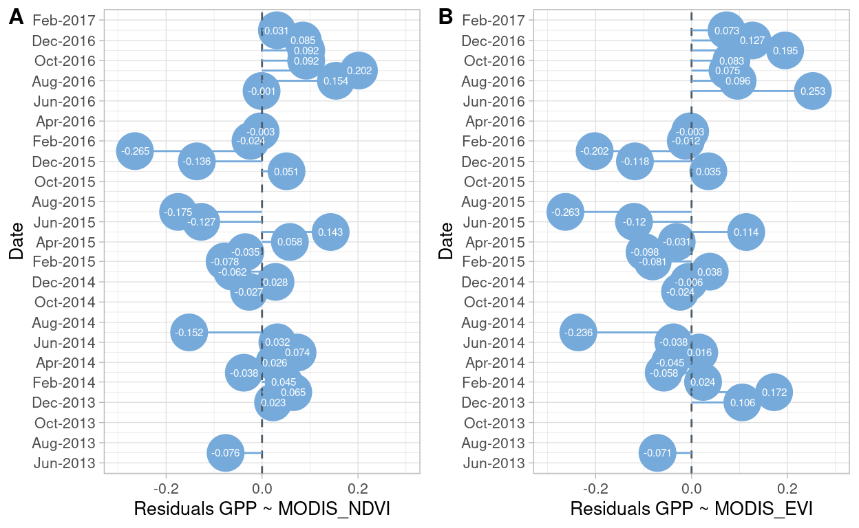
Figure 2: Residuals values for linear models GPP ~ NDVI (A) and, GPP ~ EVI (B) for registered months
Figure 2 shows the residuals values derived from the linear model between GPP with NDVI (A), and GPP with EVI (B). No patterns or consistency between months can be inferred from Figure 2.
Residuals and meteorological variables
Given that there is no clear pattern in the values of the residuals with just the months and years, I made a comparison between the values of the residuals with meteorological values per month.
- Do we have meteorological characteristics that are related to larger or shorter residuals values?
Show code
# NDVI BIOMET %%%%%%%%%%%%%%%%%%%%%%%%%%%%%%%%%%%%%%%%%%%%%%%%%%%%%%%%%%%%%%%%%%
observations_ndvi_residuals <- ndvi_observations_residuals %>%
  select(month_year, residuals) %>%
  rename(ndvi_residuals = residuals)

# EVI BIOMET %%%%%%%%%%%%%%%%%%%%%%%%%%%%%%%%%%%%%%%%%%%%%%%%%%%%%%%%%%%%%%%%%%%
observations_evi_residuals <- evi_observations_residuals %>%
  select(month_year, residuals) %>%
  rename(evi_residuals = residuals)

# Summarise biomet %%%%%%%%%%%%%%%%%%%%%%%%%%%%%%%%%%%%%%%%%%%%%%%%%%%%%%%%%%%%%
biomet_summarized <- biomet %>%
  group_by(zoo::as.yearmon(date)) %>%
  summarise(
    par_incoming = mean(par_incoming, na.rm = TRUE),
    swc = mean(swc, na.rm = TRUE),
    vpd = mean(vpd, na.rm = TRUE),
    r_h = mean(r_h, na.rm = TRUE),
    tair = mean(tair, na.rm = TRUE),
    le = mean(le, na.rm = TRUE),
    h = mean(h, na.rm = TRUE)
  ) %>%
  rename(month_year = `zoo::as.yearmon(date)`)

precipitation_summarized <- precipitation %>%
  mutate(month_year = zoo::as.yearmon(date)) %>%
  group_by(month_year) %>%
  summarize(
    total_precip = sum(precip, na.rm = TRUE)
  )

# Join datasets %%%%%%%%%%%%%%%%%%%%%%%%%%%%%%%%%%%%%%%%%%%%%%%%%%%%%%%%%%%%%%%%
residuals_biomet <- observations_ndvi_residuals %>%
  left_join(observations_evi_residuals, by = "month_year") %>%
  left_join(biomet_summarized, by = "month_year") %>%
  left_join(precipitation_summarized, by = "month_year") %>%
  select(-month_year)

tmwr_cols <- colorRampPalette(c("#91CBD765", "#CA225E"))

residuals_biomet %>%
  drop_na() %>%
  cor() %>%
  corrplot(col = tmwr_cols(200), tl.col = "black")
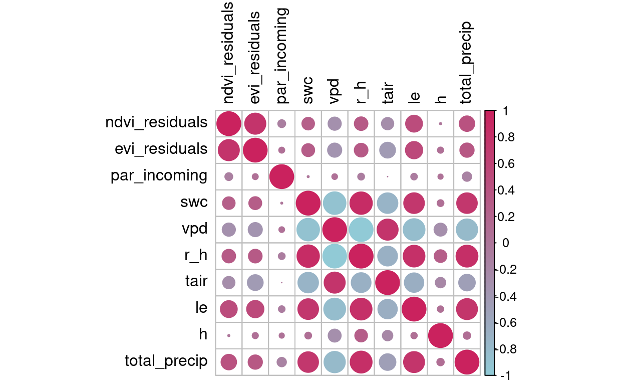
Figure 3: Correlation between the NDVI and EVI residuals with meteorological variables
- There is no a clear correlation between residuals (from NDVI and EVI) with the meteorological variables, other than Latent Heat (
le), and total precipitation per month (total_precip)
Show code
# # For EVI
# biomet_pca <- residuals_biomet %>%
#   select(-ndvi_residuals) %>%
#   drop_na() %>%
#   princomp(cor = T)
#
# biplot(biomet_pca)
#
# # For NDVI
# biomet_pca <- residuals_biomet %>%
#   select(-evi_residuals) %>%
#   drop_na() %>%
#   princomp(cor = T)
#
# biplot(biomet_pca)
Gradient analysis
In order to know which meteorological variables have more influences in the values of GPP (in-situ and MODIS) and indices, a gradient analysis (direct and indirect) was performed. Mean values for each month were calculated and those months which had no value in one of the variables were filtered out, resulting in a total of 26 observations (available months with complete values) for all the time period in this research.
Show code
# biomet_summarized contains the meteorological variables per month
# modis_indices_clean
# modis_gpp_clean

# Unite MODIS products per month and year %%%%%%%%%%%%%%%%%%%%%%%%%%%%%%%%%%%%%%
modis_gpp_month <- modis_gpp_clean %>%
  group_by(zoo::as.yearmon(date)) %>%
  summarise(
    gpp = mean(gpp, na.rm = TRUE)
  ) %>%
  rename(date = `zoo::as.yearmon(date)`)

modis_indices_month <- modis_indices_clean %>%
  group_by(zoo::as.yearmon(date)) %>%
  summarise(
    ndvi = mean(ndvi, na.rm = TRUE),
    evi = mean(evi, na.rm = TRUE)
  ) %>%
  rename(date = `zoo::as.yearmon(date)`)

modis_means <- modis_gpp_month %>%
  full_join(modis_indices_month, by = "date")

# Unite MODIS products with gpp in situ %%%%%%%%%%%%%%%%%%%%%%%%%%%%%%%%%%%%%%%%
in_situ_gpp <- monthly_gpp %>%
  mutate(date = zoo::as.yearmon(date)) %>%
  select(date, average_gpp) %>%
  rename(gpp_in_situ = average_gpp)

full_gpp <- in_situ_gpp %>%
  full_join(modis_means) %>%
  rename(gpp_modis = gpp,
         month_year = date) %>%
  full_join(biomet_summarized) %>%
  drop_na()

# Prepare data for gradient analysis %%%%%%%%%%%%%%%%%%%%%%%%%%%%%%%%%%%%%%%%%%%
rownames(full_gpp) = full_gpp$month_year
month_labels = as.factor(full_gpp$month_year)

indices <- full_gpp[ , 2:5]
meteo <- full_gpp[ , 6:12]

# NDMS execution %%%%%%%%%%%%%%%%%%%%%%%%%%%%%%%%%%%%%%%%%%%%%%%%%%%%%%%%%%%%%%%
sed <-  distance(scale(meteo), "euclidean")
out1 <-  metaMDS(sed, k = 2, trymax = 500)
scores1 <-  out1$points # generate scores
Direct gradient analysis
Show code
# Plot ordination variables %%%%%%%%%%%%%%%%%%%%%%%%%%%%%%%%%%%%%%%%%%%%%%%%%%%%
plot(scores1, col = "white")
text(scores1, labels = month_labels)
vectors1 = envfit(scores1, meteo, nperm = 0)
plot(vectors1, col = "red")

# Adding new vectors %%%%%%%%%%%%%%%%%%%%%%%%%%%%%%%%%%%%%%%%%%%%%%%%%%%%%%%%%%%
vectors2 = envfit(scores1, indices, nperm = 999)
plot(vectors2, col = "blue")
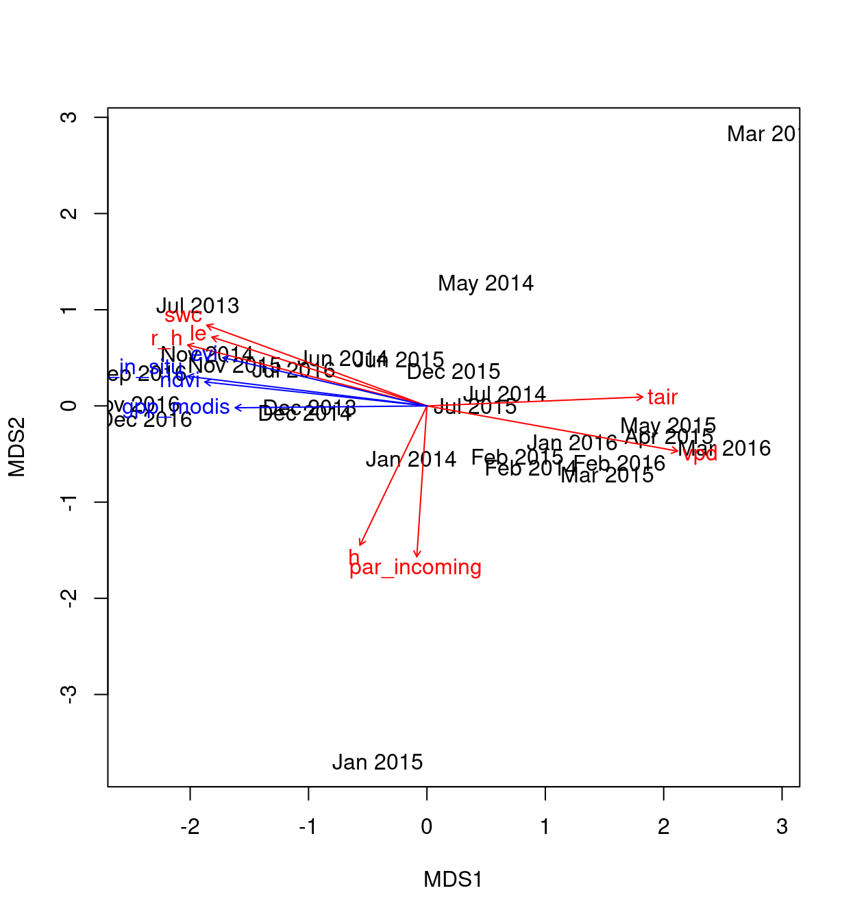
Figure 4: Direct gradient analysis
The scores for this analysis are:
Show code
vectors2
***VECTORS

                 MDS1      MDS2     r2 Pr(>r)
gpp_in_situ -0.988580  0.150676 0.9068  0.001 ***
gpp_modis   -0.999930 -0.011892 0.5689  0.001 ***
ndvi        -0.991280  0.131770 0.7767  0.001 ***
evi         -0.960060  0.279807 0.6984  0.001 ***
---
Signif. codes:  0 '***' 0.001 '**' 0.01 '*' 0.05 '.' 0.1 ' ' 1
Permutation: free
Number of permutations: 999
Indirect gradient analysis
Show code
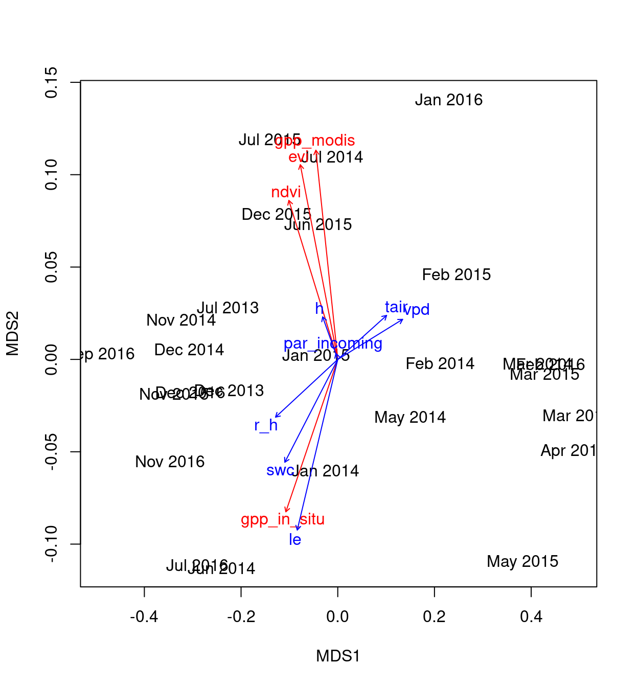
Figure 5: Indirect gradient analysis
The scores for this analysis are:
Show code
vectors4
***VECTORS

                 MDS1     MDS2     r2 Pr(>r)
par_incoming -0.77082  0.63705 0.0013  0.973
swc          -0.89135 -0.45331 0.7438  0.001 ***
vpd           0.98717  0.15967 0.9103  0.001 ***
r_h          -0.97174 -0.23603 0.8653  0.001 ***
tair          0.97331  0.22949 0.5309  0.001 ***
le           -0.67173 -0.74079 0.7671  0.001 ***
h            -0.80507  0.59318 0.0743  0.451
---
Signif. codes:  0 '***' 0.001 '**' 0.01 '*' 0.05 '.' 0.1 ' ' 1
Permutation: free
Number of permutations: 999
Conclusions
- Given data constrains (4 years of data from a single point) no further analysis could be done. Nonetheless, climate variables relations with driest months can indicate an influence on the estimations of GPP through MODIS products
- MODIS NDVI product have a better relation with GPP estimated in-situ than EVI MODIS product
- GPP derived from MODIS does not follow the seasonal patterns of GPP estimated in-situ.
- Soil water content, relative humidity and latent heat are more associated with months with higher precipitation and MODIS products.
References
James, G., Witten, D., Hastie, T., & Tibshirani, R. (2013). An introduction to statistical learning (Vol. 112, p. 18). New York: springer.